Law of Variable Proportions | Law of Diminishing Returns

The law of variable proportion is one of the fundamental laws in economics. This law deals with the short-run production function. In short run, input and output relations are studied by keeping at least some factors / inputs of production constant. The law of variable proportion states that when more and more unit of a variable input are applied with the given number / size of

number / size of the fixed inputs, the total output may initially increase at an increasing rate up to some extent, then it increases at decreasing rate, it reaches to the maximum level and ultimately it starts to decrease. This tendency of production in the short run is termed as the ‘Law of Variable Proportion’ or the Law of Diminishing Return’. This law of production exhibits the direction of the change of total product and the marginal product of the variable factor combined with fixed factors.

Different economists have offered definitions of the Law of Variable Proportion or the Law of Diminishing Return in their own way.

Alfred Marshall discussed the law of diminishing returns in relation to agriculture. He defines the law in these words “An increase in the capital and labor applied in the cultivation of land causes in general a less than proportionate increase in the amount of produce raised, unless it happens to coincide with an improvement in the arts of agriculture.”

 

Similarly, according to Prof. Leftwitch, “The law states that if the input of one resource is increased by equal increments per unit of time while the inputs of other resources are held constant, TP will increase, but beyond some point the resulting TP will increases will become smaller and smaller.”

From the definitions presented above, it is clear that the law of variable proportions or the law of diminishing returns refers to the behavior of output as the quantity of one factor is increased keeping the quantity of other factors fixed, and further it states that the marginal and average product will eventually decline.

The law of variable proportions has the following assumptions:

1. Constant Technology: The law of variable proportion assumes that the state of technology is constant. The reason is that if the state of technology changes, the marginal and average productivity of variable may rise instead of diminishing because of technological improvement.
2. Short-run: This law specially operates in the short-run because in the short run, some factors are fixed and the proportion of others has to be varied. It assumes that labor (L) is variable factor while capital (K) is the fixed factor.
3. Homogeneous Factors: This law is based on the assumption that the variable factor (labor) is applied unit by unit and each factor unit is homogeneous / identical in amount and quality.
4. Changeable Input Ratio: The law supposes that it is possible to produce output by changing the ratio of factor inputs; the ratio of fixed and variable factor is changeable; there is no fixed proportion of production function.

In the short period of time, capital is held constant in manufacturing while in agriculture land is held constant and other inputs are used in varying number. The law of variable proportions or the law of diminishing returns is illustrated with the help of hypothetical data given in table. In the illustration, labor service is supposed as a variable factor.

No. of Labor	Total Product	Marginal Product	Average Product	Stage of Returns
(L)	(TPL)	APL=TPL/L	MPL=∆TPL/∆L
1 2 3 4 5 6 7 8 9 10 11	8 22 39 52 60 66 70 72 72 70 66	8 11 13 13 12 11 10 9 8 7 6	8 12 17 13 8 6 4 2 0 -2 -4	1st Stage 2nd Stage 3rd Stage

The data in table show that production changes due to change in variable factor (labor). As the number of labor is increased, initially, both marginal and average product of labor increases. After employing more of labor, both APL and MPL falls more rapidly. Falling in the APL and MPL will continue as more labor is put in the production. Hiring of 9th unit of labor adds only nominal amount of output on iron industry. After then, the additional unit of labor i.e., 10th unit, the marginal product becomes negative. Here after, production becomes less.

The operation of the law of variable proportion can be explained in the following figure.

Three Stages of Variable Proportions

The vertical axis of the both figure shows the total, average and marginal product of the variable factor and the horizontal axis shows the units employed of the variable factor. The quantity of variable factor is increased relative to the fixed factors, there may arise three different stages.

First Stage

This stage covers the production ranges OL2 units of labor. In the first stage, total product (TP) increases at increasing rate up to the point A (i.e., called point of inflexion) after then TP increases at diminishing rate. At that movement of operation, MPL increases till the use of OL1 unit of labor and begins to decline whereas APL continuously increases till OL2 unit of labor. In this stage, MPL is greater than APL. MPL and APL become equal at OL2 units of labor employed, as shown by the point B. Point B is the end of this stage and the second stage starts.

Causes of returns in stage first

1. Increase in efficiency of fixed factor: In the initial stage, the quantity of fixed factor is abundant in comparison to the quantity of variable factor. As more units of variable factors are added to the constant quantity of fixed factor than the fixed is more intensively and effectively utilized i.e., the efficiency of fixed factors are added to it.
2. Increase in efficiency: In the initial stage, we get increasing returns because as more units of the variable factors are employed, the efficiency of the variable factors itself increases. The reason of efficiency is that with sufficient quantity of variable factor, introduction of division of labor and specialization becomes possible which result in higher productivity.

Second Stage

This stage covers the production ranges between OL2 and OL3 units of labor. In this stage, both MPL and APL decline but positive. However, MPL declines at the faster rate. It is important to note that, at OL3 unit of labor, TP becomes maximum as shown by the point M in figure (A) and MPL becomes zero level at point OL3.

Causes of returns in stage second

1. Scarcity of fixed factor: In the short-run, the quantity of fixed factor cannot be varied. For this reason, the further increases in the variable factor will cause marginal and average product to decline because the fixed factor then becomes inadequate relative to the quantity of variable factor.
2. Indivisibility of fixed factor: If the fixed factors are perfectly divisible, there no change in proportion or increasing and decreasingly returns. In short-run, the size of plant is being unchanged, so the fixed factors are indivisible. Therefore, the excess variable factor are used in combination with indivisible fixed factor, the average product of variable factor diminishes.
3. Imperfect substitutability of the factors: The operation of law of diminishing returns is the imperfect substitutability of one factor for another. The perfect substitute of the scarce fixed factor been available, then the capacity of the scarce fixed factor during the 2nd stage would have been made up by increasing the supply of the perfect substitute with the result that output could be expended without diminishing returns.

Third Stage

Third stage begins with the decline in TPL. As the figure shows, the use of labor in excess of OL3 cause decline in TPL and negative MPL because of overcrowding of labor. However, APL will be positive i.e., tends to zero but not becomes zero.

Causes of returns in third stage

1. Too excessive amount of fixed factor: As the amount of the variable factor continue to be increased to constant quantity of the other; a stage is reached when the total product declines and marginal product become negative. This is due to the fact that the quantity of variable factor becomes too excessive relative to the fixed factor so that they affect each other’s efficiency.

  You may also like to read:               

• Production Function

• Firm determines the best level of output and price for products

• Law of Demand: Higher the price, the smaller the quantity demanded

• Law of Substitution, Equi-marginal Principle

•  Demand | Theory of Demand: desire, willingness and ability to pay for a commodity

• Elasticity of Demand: Types of Price Elasticity of Demand

• Law of Diminishing Marginal Utility

• Uses of Price Elasticity of Demand in Managerial Decision-making

Production Function | Linear Production Function | Quadratic Production Function | Cubic Production Function | Power Production Function

Production involves the transformation of inputs into outputs. Production involves the transformation of inputs into physical output. The output is thus, a function of factors which are also called inputs. The term ‘production function’ refers to the relationship between the inputs and outputs produced by them. The functional relationship between physical inputs and physical output of a firm is known as production function. Algebraically, production function can be expressed as,

Q = f ( Ld, L, K, M…. )

Where, 

Q stands for the quantity of output, Ld, L, K and M stand for the land, labor, capital and management respectively.

The above equation shows that the quantity (Q) of output produced depends upon the quantities of the factors used. Simply, production function expresses the relationship between the quantity of output and the quantities of the various inputs used for the production. More precisely, the production function states the maximum quantity of output that can be produced with by given quantities of various inputs.

In economic theory, there are two types of production functions on time basis. The production function when the quantities of some inputs such as capital and labor are kept constant and the quantity of one input such as labor is varied. This kind of production function [Q = f (K, L)] is known as short-run production function. The study of short-run production function is the subject-matter of the law of diminishing returns which is also called the law of variable proportion.

Secondly, we study production function (input – output relation) by varying all inputs, and this is called long-run production function and can be expressed as Q = f (Ld, L, K, M ). This form is the subject-matter of the law of returns to scale. Generally, the terms constant and increasing returns are used with reference to constant and increasing returns to scale.

Besides these, there are other production function, such as

1) Linear Production Function

A linear production function would take the form:

Total production Y = a + bx

From this, function for the managerial production will be,

= Y / X.a / x + b

The equation for the marginal product will be,

∆Y / ∆X = b

2) Power Function

A power function expresses output Y, as a function of input in the form:

y = AX^α

It contains certain properties:

a) The exponents are the elasticity of production. Thus, in the above function, the exponent α represents the elasticity of production.

b) The equation is linear in the logarithms, i.e., it can be expressed as, 

log Y = logA + αlogX

when the power function is expressed in logarithmic form as above, the coefficient α represents the elasticity of production.

c) If one input is increased while all others are held constant, marginal product will be decline.

3) Quadratic Production Function

The production function may be quadratic, taking the following form:

Y = a + bx – cx²

Where, the dependent variable Y shows total output and the independent variable X represents input. The small letters are parameters; their probable values are determined by a statistical analysis of the data.

Properties of quadratic function:

a) The minus sign in the last term denotes diminishing marginal returns.

b) The equation allows for decreasing marginal product but not for both increasing and decreasing marginal products.

c) The elasticity of production is not constant at all points along the curve as in a power function, but declines with input magnitude.

d) The equation never allows for an increasing marginal product.

4) Cubic Production Function

The cubic production function takes the following form:

Y = a + bx + cx² – dx³

Some important special properties of a cubic production function are:

a) It allows for both increasing and decreasing marginal productivity.

b) The elasticity of production varies at each point of the curve.

c) Marginal productivity decreases at an increasing rate in the later stages.

5) Power Production Function (Cobb-Douglas Function)

Power functions have been employed in a large number of empirical production studies, particularly since Charles W. Cobb and Paul H. Douglass’s pioneering work in the late 1920s. The impact of this work was so great that power production functions are now frequently referred to as Cobb-Douglas production functions.

Cobb-Douglas production function can be expressed as,

Q = AK^α L^β

Where, Q = total output

L = index of employment of labor in manufacturing

K = index of fixed capital in manufacturing

The exponents α and β are the elasticities of production i.e., α and β measure the percentage response of output to percentage changes in labor and capital respectively.

Properties of Power Function:

a) Power functions allow the marginal productivity of a given input to depend upon the levels of all inputs employed a condition that often holds in actual production systems.

b) They are linear in logarithms and thus can be easily analyzed using linear regression analysis.

log Q = log A + α log K + β log L

The least squares technique can be used to estimate the coefficients of equation and thereby the parameters of equation.

c) Power functions facilitate returns to scale estimation. Returns to scale are easily calculated by summing the exponents of the power function. If the sum of the exponent is less than one, (α + β < 1) diminishing returns are included. A sum greater than one (α + β > 1) indicates increasing returns. Finally, if the sum of the exponent is exactly one (α + β = 1), returns to scale are constant.

 You may also like to read:                    

• Law of Variable Proportions | Law of Diminishing Returns

• Law of Returns to Scale in Production | Increasing Returns to Scale | Constance Returns to Scale | Decreasing Returns to Scale

• Production of maximum output in the firm | Production of a given output at minimum cost | Production of maximum output with a given level of cost

• Derivation of Market Supply Curve and Shift in the Supply Curve

• Development of the Marketing Concept | Production Concept, Product Concept, Selling Concept, Marketing Concept and Societal Marketing Concept

• Elasticity of Demand: Types of Price Elasticity of Demand

• Uses of Price Elasticity of Demand in Managerial Decision-making

Profit Maximization Objective of a Firm | Total Revenue (TR) - Total Cost (TC) Approach | Marginal Revenue (MR) - Marginal Cost (MC) Approach

Profit maximization is the most accurate description of managerial goal. The profit maximization is one of the very important assumptions of economic theory, which always assumes that a firm aims to maximize profit. The attempt of an entrepreneur to maximize profit is regarded as a rational behavior. Hence, profit maximization continues to be a central concept in managerial economics.

There are two approaches to explain the equilibrium of a firm on the context of profit maximization. Among them one is old method of total cost and total revenue approach and another is the marginal revenue and marginal cost approach.

Total Revenue (TR) – Total Cost (TC) Approach

Total revenue (TR) and total cost (TC) approach is the simplest method to determine the equilibrium of a firm. To calculate the profit of a firm, we find out the difference between the total revenue and total cost at difference levels of output. A firm is said to be in equilibrium when the difference between total revenue (TR) and total cost (TC) is maximum. Every rational producer will try to maximize his profit. We can find equilibrium of a firm with the help of this approach both under perfect and imperfect (monopoly) market competition.

i) Equilibrium of the firm under perfect competition

The firm is in equilibrium when it has no incentive to change its level of output. In perfect competition, a firm is said to be in equilibrium when it maximizes its profits (π), which is defined as the difference between total revenue and total cost.

 

π = TR – TC

Where,

π = profit,

TR = Total Revenue and

TC = Total Cost

Given that the normal profit rate is included in the cost items of the firm, π is the profit above the normal rate of return on capital and the remuneration for the risk bearing function of the entrepreneur. The firm is in equilibrium when it produces the output that maximized the differences between total receipts (Revenue) and total costs. The equilibrium of the firm can be explained with the help of the following figure:

As shown in the figure, TR and TC are total revenue and total cost curves of a firm in a perfectly competitive market. TR curve in a straight line through the origin, showing that the price is constant at all levels of output. The firm is a price taker and can sell any amount of output at the going market price, with its TR increasing proportionately with its sales. The slope of TR curve is the MR. It is constant and equal to the prevailing market price. Since all units are sold at the same price.

The slope of TC curves reflects ‘U’ shape of the AC curve i.e. law of variable proportions. The firm maximizes its profit at the output ‘OX’, where the distance between TR and TC is the greatest. At the lower (OX1) and higher levels (OX2) than OX, the firm has losses. The TR-TC approach awkward to use when firms are combined together in the study of the industry.

ii) Equilibrium of the Firm under Imperfect Competition (Monopoly)

Under imperfect competition, AR and MR of a firm are two different things. This is because under imperfect competition, a firm is a price-maker. It can sell more by lowering the price of its output. In the figure, AR and MR curves of a firm fall downward from left to right. According to this approach, for a firm to be equilibrium or maximization of profit, marginal revenue should be equal to marginal cost and the marginal cost curve should cut the marginal revenue curve from below.

 

It is shown in the figure, at the beginning, total cost is higher than total revenue. There is no profit. At points P and Q, total revenue is equal to total cost. So, there is neither profit nor loss and is called the break-even point. After OA output, total revenue is higher than total cost, so profit begins to show. At OB output, the difference between total revenue and total cost is maximum. The firm is in equilibrium and earns maximum profit, TR - TC (EB - NB) = EN is profit. Point Q is again the break-even point. Beyond OC output, total cost exceeds total revenue and the firm incurs losses. In case of perfect competition, the TR become the straight line.

 

Marginal Revenue (MR) - Marginal Cost (MC) Approach

Marginal revenue and marginal cost approach is another method to know the equilibrium of a firm. The modern economist Mrs. John Robinson propounded this approach. According to this approach, for a firm to be equilibrium or maximization of profit, marginal revenue (MR) should be equal to marginal cost (MC) and the marginal cost curve should - cut the marginal revenue curve from below. It will be profitable for a firm to increase its production when MR exceeds MC.

i) Equilibrium of the firm under perfect competition

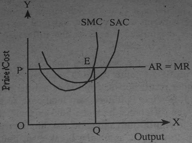
The equilibrium of a firm in the perfect competition can also be shown through the help of marginal revenue (MR) and marginal cost (MC) approach. For fulfilling the condition of maximum profit, marginal cost (MC) must be less than marginal revenue (MR). A firm is said to be in equilibrium when marginal cost (MC) must be equal to the marginal revenue (MR) or MC curve must intersect MR curve from below. It is shown in the figure:

In the figure, AR and MR are the same and AR = MR is a straight line. It is assumed that MC falls at first and then starts rising. MC curve cuts MR curve at E point from below and it is equal to MR. The profit maximizing output is OQ where firm fulfills two basic conditions of equilibrium.

ii) Equilibrium of a firm under imperfect competition (Monopoly)

Under imperfect competition, AR and MR of a firm are two different things. This is because under imperfect competition, a firm is a price-maker. It can sell more by lowering the price of its output. In the figure, AR and MR curves of a firm fall downward from left to right. According to this approach, for a firm to be equilibrium or maximization of profit, marginal revenue should be equal to marginal cost and marginal cost curve should cut the marginal revenue curve from below.

 

In this figure, at point E both the conditions of equilibrium have been fulfilled. Hence, E is the point of equilibrium. The firm gets equilibrium at OM output where marginal revenue is equal to marginal cost. The OM quality of output is sold at price OP price. Before OM output, the increase in output add more to revenue than to cost but after OM output, the increase in output adds more to cost than revenue. Profit is the total revenue OMQP minus total cost OMNR. Hence, the firm earns the abnormal profit equal to RNQP.

Criticisms/ Demerits of Profit Maximization Theory

The objective has been criticized by some economists saying there may have other objectives in a firm such as sales maximization, welfare or satisfactions etc. This objective is criticized on the following grounds.

1. Profit maximization criterion is vague and ambiguous. Profit may be long-term, after tax or before tax. It is not clear.
2. In this objective, total profit earned during the life of assets and timing of their realization is ignored. Hence, equal value for earning realized on different periods is not realistic. It ignores the time value of money.
3. This objective is concerned only with the size of profit and gives no weight to the degree of uncertainty of future profits. Two businesses with varying degree of risk and producing same size of profit is considered similar under profit maximization criterion. Thus, the risk element is ignored, which is one of the most important dimensions of financial management.
4. This objective is incomplete because it ignores the appreciation in the value of securities or firm. Investors and owners of the businessmen are benefited not only by the earning of profit, but also due to the appreciation in the stock price.

  SOME RELATED LINKS  

• Modern Oligopolistic firms typically seek to maximize their sales subject to minimum profit constraints | Boumol's Theory of Sales Maximization

• Pricing decision on the basis of Cost Plus Pricing Theory

• Reasons behind aiming at reasonable profit rather than maximum profit by most of firms

• Value of Maximization Theory of Firm | Superiority of Maximization Theory

• H. A. Simon opines that firms aim at satisfying rather than maximizing profit | Simon's Satisficing Theory